How to Apply Conditional Formatting in a Power BI Area Chart (2026)

Contoso’s sales director wanted the monthly revenue trend to turn orange whenever a month fell below the $250K target, so nobody had to read the axis to spot a weak month. For years, area chart conditional formatting in Power BI simply didn’t exist, and people used a column chart trick to fake it.

That changed in mid-2026. Line and area charts now have a real fx button on the line color, and the shaded area follows those colors. In this tutorial, I’ll show you how to color an area chart with rules, a gradient and a DAX measure, using a Contoso sales table with monthly revenue for 2025 and 2026.

Quick answer: Select the area chart, open Format visual > Lines > Color, and select fx. Choose a Format style (Gradient, Rules or Field value), base it on your measure, and select OK. The line and the shaded area under it change color by value. It works only when the chart has a single series (no Legend field).

What you can conditionally format in an area chart

The area chart shares its formatting with the line chart, so the same options apply:

Setting	Where	What changes
Line and area color	Lines > Color > fx	Each segment of the line and the shading under it
Marker color	Markers > Color > fx	The dot on each data point (markers are off by default)
Data label color	Data labels > Values > Color > fx	The value text on each point

All of them offer the three standard format styles: Gradient, Rules and Field value. If you’ve used them in tables before, they work the same way here; the Power BI conditional formatting guide covers the dialog in depth.

Before you start: one series only

Conditional colors on lines work only when the chart has one series. If you add a field to the Legend well, or a second measure to the Y-axis, Power BI turns segment coloring off and you’re back to one color per series.

My chart has Month on the X-axis and Sum of Revenue on the Y-axis, nothing else. If you need several series with a highlight, the closest native option is a stacked chart with fixed colors; the post on conditional formatting in a stacked column chart shows how that behaves with a legend.

Method 1: Color the area with rules

Rules are the best fit for a target, because the color changes at an exact number.

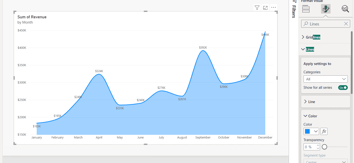
1. Select the area chart and open Format visual > Visual. Typing Lines in the Format pane search box gets you there fast.
2. Expand Lines, then the Color section, and select the fx button next to the color swatch.

1. In the Color – Categories dialog, set Format style to Rules.
2. Under What field should we base this on?, pick Sum of Revenue. Summarization changes to Sum.
3. First rule: If value >= 0 Number and < 250000 Number, then orange.
4. Select New rule. Second rule: >= 250000 Number and < 1000000 Number, then dark blue.
5. Select OK.

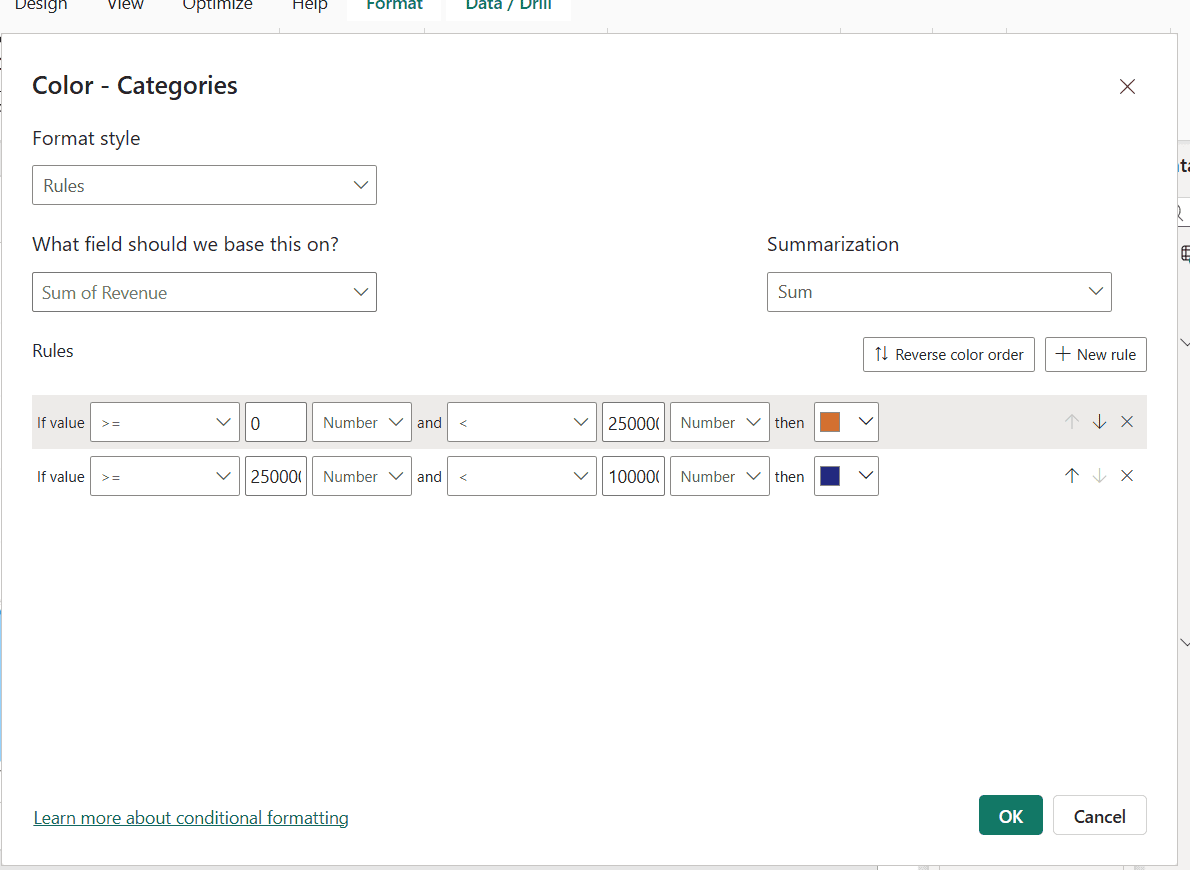
Watch the value type. New rules default to Percent, which means a percent of the range between the lowest and highest month, not dollars. Switch each one to Number when you type real amounts.

Here’s the result. January to March, May and June are under $250K and turn orange, while April and July through December stay blue:

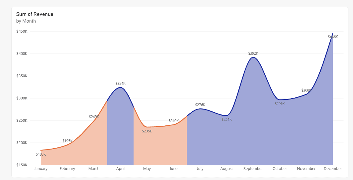
The color changes halfway between two points, because Segment type under Lines > Color is set to Center by default. Choose Left or Right to move the color change toward one end of the segment. A Gradient toggle also appears; turn it off for hard color edges.

Method 2: Use a gradient

A gradient works better when you want to show how high or low each month is, not just pass or fail. In the same dialog, set Format style to Gradient and base it on Sum of Revenue. Pick a color for Minimum (Lowest value) and Maximum (Highest value).

Check Add a middle color if you want a third color in the center.

You can type a Custom number for the minimum and maximum instead of the lowest and highest values. That keeps colors stable when filters change the data. The same idea is used to apply conditional formatting to a gauge chart, if you want a matching KPI next to the trend.

Method 3: Field value with a DAX color measure

When the color logic is complex, for example comparing to a target that changes each month, write a measure that returns a color:

Revenue Color =
IF (
    SUM ( Sales[Revenue] ) >= 250000,
    "#12239E",   -- dark blue: on or above target
    "#E66C37"    -- orange: below target
)

Then open Lines > Color > fx, set Format style to Field value, and pick Revenue Color. The measure must return text: a hex code, a CSS color name such as red, or a theme name such as good or bad. If you need help with the IF logic, see these Power BI measure IF examples.

You can point the comparison at another measure, such as a Target measure, instead of a fixed 250000. That’s the cleanest way to color by target when the target differs by month or region.

Color the markers and labels too

Markers are off by default on area charts. Turn on Markers in Format visual, expand Color, and select its fx to use the same rules or measure.

A common trick is a Field value measure that returns a color only for the highest and lowest months and "#FFFFFF00" (fully transparent) for the rest, so only two markers show.

Data labels have their own fx under Data labels > Values. If you also want a lighter fill, the post on area chart transparency in Power BI covers the Transparency slider.

The old workaround (before 2026)

Older tutorials, including the first version of this one, built a column chart, set Columns > Color > fx, and then switched the visual to an area chart so the marker colors carried over.

You don’t need that anymore. It only colored markers, never the area, and the colors could reset when you edited the visual. If you still need column colors by value, see how to create a Power BI bar chart with conditional colors.

Troubleshooting

• No fx button next to Lines > Color: update Power BI Desktop. Conditional formatting for line charts became generally available in mid-2026.
• The fx button is there but colors don’t change: the chart has a Legend field or two measures. Remove them so there’s one series.
• Every month has the same color: the rules use Percent instead of Number, or the ranges don’t cover your values.
• The color switches between points, not at them: change Segment type from Center to Left or Right.
• Field value does nothing: the measure returns a number instead of text, or a misspelled color name.

If you’re formatting other charts in the same report, start with these:

• Area Chart in Power BI
• Power BI Pie Chart Conditional Formatting
• Power BI Matrix Visual Conditional Formatting
• How to Create a Stacked Column Chart in Power BI (and a Stacked Bar Chart)

Frequently Asked Questions